
Math Modeling
In the fall 2012, I used the textbook "Mathematical Modeling" (3rd Edition) by Meerschaert (http://www.stt.msu.edu/~mcubed/modeling.html). Notice that the 4th edition has just come out. Overall this is a good book to introduce math modeling to undergraduates from different majors because the material is a nice balance of math theory, computer programming and applications to a variety of fields (such as biology, economics and physics). Following are some basic problems from this book that I required my students to master. Please refer to the book for details on the related theory and similar exercises.
1) Initial Value Problem
*** Question 2: To further simplify the problem, consider that the effect of competition is relatively small, such as 1e-7. Find the equilibrium points and plot the vector field for this problem.
*** Question 3: Use the eigenvalue method to test the stability of each equilibrium. Can the two populations of whales grow to stable equilibrium starting from their current levels?
*** Question 4: If both populations of whales will eventually grow back to their natural levels in the absence of any further harvesting, how long will this take?
*** Question 5: What happens to the model if we use too large of a time step in the forward Euler method as we simulate the whale populations with respect to time?
Note: I will include some sensitivity analysis for this model in the future.
TYPE 2:
(Example 5.3) Consider the electrical circuit diagrammed in the following figure:
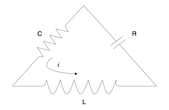
The circuit consists of a capacitor, a resistor, and an inductor in a simple closed loop. The effect of each component of the circuit is measured in terms of the relationship between current and voltage on that branch of the loop. An idealized
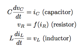
physical model gives the relations where vC represents the voltage across the capacitor, iR represents the current through the resistor, and so on. The function f(x) is called the v-i characteristic of the resistor. Usually f(x) has the same sign as x. This is called a passive resistor. Some control circuits use an active resistor, where f(x) and x have opposite sign for small x. In the classical linear model of the RLC circuit, we assume that f(x) = Rx where R > 0 is the resistance. Kirchoff’s current law states that the sum of the currents flowing into a node equals the sum of the currents flowing out. Kirchoff’s voltage law states that the sum of the voltage drops along a closed loop must add up to zero. Determine the behaviors of this circuit over time under the effect of varying the capacitance C over the entire range 0 < C < infinity, and f(x) = x3 + 4x by:
*** sketching the phase portrait for the linear system to illustrate the equilibrium and solution curves.
*** solving the linear system by the method of eigenvalues and eigenvectors.
Note: I will include some sensitivity analysis for this problem in the future.
3) Constrained Optimization: Lagrange multipliers
(Example 2.2) Reconsider the color TV problem above. There we assumed that the company has the potential to produce any number of TV sets per year. Now we will introduce constraints based on the available production capacity. Consideration of these two new products came about because the company plans to discontinue manufacture of some older models, thus providing excess capacity at its assembly plant. This excess capacity could be used to increase production of other existing product lines, but the company feels that the new products will be more profitable. It is estimated that the available production capacity will be sufficient to produce 10,000 sets per year (≈ 200 per week). The company has an ample supply of 19–inch and 21–inch LCD panels and other standard components; however, the circuit boards necessary for constructing the sets are currently in short supply. Also, the 19–inch TV requires a different board than the 21–inch model because of the internal configuration, which cannot be changed without a major redesign, which the company is not prepared to undertake at this time. The supplier is able to supply 8,000 boards per year for the 21–inch model and 5,000 boards per year for the 19–inch model. Taking this information into account, how should the company set production levels?
Note: I will include some sensitivity analysis for this problem in the future.
4) Linear Programming
(Example 3.4) A family farm has 625 acres available for planting. The crops the family is considering are corn, wheat, and oats. It is anticipated that 1,000 acre–ft of water will be available for irrigation, and the farmers will be able to devote 300 hours of labor per week. Additional data are presented below.
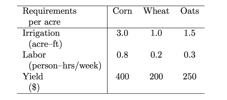
Use a computer algebra system to answer to the following questions:
*** Question 1: Find the amount of each crop that should be planted for maximum profit.
*** Question 2: What will be the effect of one additional acre–ft of irrigation water on the optimal solution?
*** Question 3: What will be the effect of a slightly higher yield for corn ($450 instead of $400) on the optimal solution?
*** Question 4: What will be the effect of a slightly higher yield for oats ($260 instead of $250) on the optimal solution?