
Numerical Analysis
In the spring 2013, I used the textbook "Numerical Analysis" (9th Edition) by Burden and Faires. I think the students liked the book because the algorithms for the numerical methods were easy enough to understand and implement as well as the examples were explained clearly and served as great validations for their code. However some of the math theory or derivation behind the numerical methods can be quite challenging for undergraduates to grasp. Following are some of the numerical methods which were implemented in Matlab by my students and under my guidance. All the programs have been validated with the examples in the textbook.
*** Root-finding Method
- Bisection Method (http://en.wikipedia.org/wiki/Bisection_method)
***Algorithm 2.1 (p. 49) in "Numerical Analysis" (9th Edition) by Burden and Faires
***Example 1 (p. 50): Show that f(x) = x^3+4*x^2-10 = 0 has a root in [1,2], and use the Bisection method to determine an approximation to the root that is accurate to at least within 10^(-4).
func = inline('x^3+4*x^2-10'); %given function f(x)
a = 1; %first endpoint of the interval
b = 2; %last endpoint of the interval
tol = 10^-4;  %tolerance for the accuracy
n = 14; %maximum number of iterations

i = 1;
FA = func(a);

while i <= n
    p = a + (b-a)/2;
    FP = func(p);
    if FP == 0 || (b-a)/2<tol
        disp(p);
        break
    end
    i = i+1;
    if FA*FP>0
        a = p;
        FA=FP;
    else
        b = p;
    end
end
p
- Fixed-point Iteration (http://en.wikipedia.org/wiki/Fixed-point_iteration)
***Algorithm 2.2 (p. 60) in "Numerical Analysis" (9th Edition) by Burden and Faires
***Problem 11 (p. 65): Use the fixed-point iteration to find a root of the equation x = g(x) where g(x) = (2 - e^x + x^2)/3.
g = inline('(2-exp(x)+x^2)*(1/3)');
p0 = 0 %initial approximation
tol = 10^-5; %tolerance for the accuracy
n = 14;  %maximum number of iterations

i = 1;

while i <= n
    p = vpa(g(p0),6)
    i
    if abs(p-p0) < tol
        disp(p);
        break
    end
    i = i+1;
   p0 = p;
end
vpa(p,6)
- Newton's Method (https://en.wikipedia.org/wiki/Newton%27s_method)
***Algorithm 2.3 (p. 68) in "Numerical Analysis" (9th Edition) by Burden and Faires
***Example 1 (p. 69): Show that g(x) = cos(x) - x = 0 has a root using Newton's method to determine an approximation to the root that is accurate to at least within 10^(-5).
g = inline('cos(x)-x');

syms x;
diff(g(x))

p0 = 0.5;  %initial approximation
tol = 10^-5;   %tolearance of the accuracy
n = 300;  %maximum number of iterations

i = 1;

while i <= n
    p = vpa(p0 - g(p0)/subs(diff(g(x)),p0), 10)
    if abs(p-p0) < tol
        i
        disp(p);
        break
    end
    i = i+1;
    p0 = p;
end
p
- Secant method (http://en.wikipedia.org/wiki/Secant_method
***Algorithm 2.4 (p. 72) in "Numerical Analysis" (9th Edition) by Burden and Faires
***Problem 6 (p. 75): Show that g(x) = e^x + 2^(-x) + 2cos(x) - 6 = 0 has a root lies between 1 and 2 using the secant method to determine an approximation to the root that is accurate to at least within 10^(-5).
g = inline('exp(x)+2^(-x)+2*cos(x)-6');
p0 = 1;  %initial approximation
p1 = 2;   %initial approximation
tol = 10^-5;    %tolerance for accuracy
n = 14;   %maximum number of iterations

i = 2;
q0 = vpa(g(p0),10);
q1 = vpa(g(p1),10);

while i <= n
    p = vpa(p1 - q1*(p1-p0)/(q1-q0), 10)
    if abs(p-p1) < tol
        disp(p);
        break
    end
    i = i+1;
    p0 = p1;
    q0 = q1;
    p1 = p;
    q1 = vpa(g(p),10);
end
p
*** Interpolation and Polynomial Approximation
- Lagrange Polynomial (http://en.wikipedia.org/wiki/Lagrange_polynomial
***Example (p. 105): A census of the population of the United States is taken every 10 years. The following table lists the population, in thousands of people, from 1950 to 2000, and the data are also represented in the following figure.
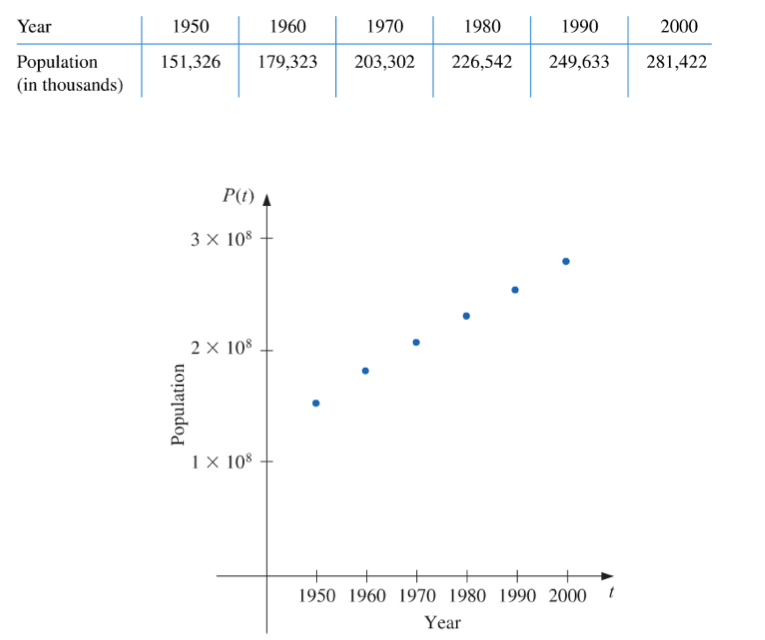
Use Lagrange interpolation to approximate the population in the years 1940, 1975, and 2020.
*Lagrange polynomials
Lo = inline('(x-1960)*(x-1970)*(x-1980)*(x-1990)*(x-2000)/-12000000');
L1 = inline('(x-1950)*(x-1970)*(x-1980)*(x-1990)*(x-2000)/2400000');
L2 = inline('(x-1950)*(x-1960)*(x-1980)*(x-1990)*(x-2000)/-1200000');
L3 = inline('(x-1950)*(x-1960)*(x-1970)*(x-1990)*(x-2000)/1200000');
L4 = inline('(x-1950)*(x-1960)*(x-1970)*(x-1980)*(x-2000)/-2400000');
L5 = inline('(x-1950)*(x-1960)*(x-1970)*(x-1980)*(x-1990)/12000000');

*Data input
x = [1950 1960 1970 1980 1990 2000];
y = [151326 179323 203302 226542 249633 281422];

P1940 = Lo(1940)*y(1)+L1(1940)*y(2)+L2(1940)*y(3)+L3(1940)*y(4)+L4(1940)*y(5)+L5(1940)*y(6)
P1975 = Lo(1975)*y(1)+L1(1975)*y(2)+L2(1975)*y(3)+L3(1975)*y(4)+L4(1975)*y(5)+L5(1975)*y(6)
P2020 = Lo(2020)*y(1)+L1(2020)*y(2)+L2(2020)*y(3)+L3(2020)*y(4)+L4(2020)*y(5)+L5(2020)*y(6)

*Expands polynomial
x = sym('x')
Lo = sym('(x-1960)*(x-1970)*(x-1980)*(x-1990)*(x-2000)/-12000000');
L1 = sym('(x-1950)*(x-1970)*(x-1980)*(x-1990)*(x-2000)/2400000');
L2 = sym('(x-1950)*(x-1960)*(x-1980)*(x-1990)*(x-2000)/-1200000');
L3 = sym('(x-1950)*(x-1960)*(x-1970)*(x-1990)*(x-2000)/1200000');
L4 = sym('(x-1950)*(x-1960)*(x-1970)*(x-1980)*(x-2000)/-2400000');
L5 = sym('(x-1950)*(x-1960)*(x-1970)*(x-1980)*(x-1990)/12000000');
y = Lo*y(1)+L1*y(2)+L2*y(3)+L3*y(4)+L4*y(5)+L5*y(6)
expand(y)
- Divided Differences (http://en.wikipedia.org/wiki/Divided_differences)
*** For the same example of the census of the population of the United States, use appropriate divided differences to approximate the population in the years 1940, 1975, and 2020.
%Clear workspace
clear

%Inputs
n = 6; %Number of data points
c = 1940; %Value you want to approximate

%Calculated setup
N = n-1; %Degree of the polynomial
F = zeros(N+1,N+1); %initializes array of divided differences

%Note: to make backwards difference, order the points descending
%For forward difference, order the points ascending
x = [1950 1960 1970 1980 1990 2000];
F(1,1) = 151326;
F(2,1) = 179323;
F(3,1) = 203302;
F(4,1) = 226542;
F(5,1) = 249633;
F(6,1) = 281422;

for(i = 2:N+1)
   for(j = 2:i)
      F(i,j) = (F(i,j-1)-F(i-1,j-1))/(x(i)-x(i-j+1));
   end
end

format long

F

Poly = F(1,1);
for i = 2:N+1
    p = 1;
    for j = 1:i-1
      p=p*(c-x(j));
      end
    Poly = Poly + F(i,i)*p;
end
format long
Poly
- Cubic Spline Interpolation (http://en.wikipedia.org/wiki/Spline_interpolation)
***Algorithm 3.4 (p. 149) in "Numerical Analysis" (9th Edition) by Burden and Faires
***Example 2 (p. 150): Use the data points (0,1), (1,e), (2,e^2) and (3,e^3) to form a natural cubic spline S(x) that approximates f(x) = e^x.
n = 3;  %number of data points - 1
x = zeros(n+1,1);
a = zeros(n+1,1);

%(x(i), a(i)) are the given data points
x(1) = 0;
x(2) = 1;
x(3) = 2;
x(4) = 3;

a(1) = 1;
a(2) = exp(1);
a(3) = exp(2);
a(4) = exp(3);

b = zeros(n+1,1);
c = zeros(n+1,1);
d = zeros(n+1,1);
h = zeros(n+1,1);
alpha = zeros(n+1,1);
l = zeros(n+1,1);
mu = zeros(n+1,1);
z = zeros(n+1,1);

for i = 1:n
    h(i) = x(i+1) - x(i);
end

for i = 2:n
    alpha(i) = 3*(a(i+1)-a(i))/h(i) - 3*(a(i)-a(i-1))/h(i-1);
end

l(1) = 1;

for i = 2:n
    l(i) = 2*(x(i+1)-x(i-1))-h(i-1)*mu(i-1);
    mu(i) = h(i)/l(i);
    z(i) = (alpha(i)-h(i-1)*z(i-1))/l(i);
end

l(n+1) = 1;
z(n+1) = 0;
c(n+1) = 0;

for j = n:-1:1
    c(j) = z(j) - mu(j)*c(j+1);
    b(j) = (a(j+1)-a(j))/h(j) - h(j)*(c(j+1)+2*c(j))/3;
    d(j) = (c(j+1)-c(j))/(3*h(j));
end

a
b
c
d
*** Numerical Differentiation (http://en.wikipedia.org/wiki/Finite_difference)
- Forward Difference
*** Problem 8d (p. 183): Use the forward-difference formulas to approximate the derivatives of f(x) = [cos(3x)]^2 - e^(2x) at x_0 = −2.3 using h = 0.2, h = 0.1 and h = 0.05. Which values of "h" gives the best approximation to the true derivative of f(x)?
f=inline('(cos(3*x))^2 - exp(2*x)');
h=[.2,.1,.05];

for i=1:3
   h(i)
   forward_diff=(f(-2.3+h(i))-f(-2.3))/h(i)
end
- Backward Difference
***Problem 8d (p. 183): Use the backward-difference formulas to approximate the derivatives of f(x) = [cos(3x)]^2 - e^(2x) at x_0 = −2.3 using h = 0.2, h = 0.1 and h = 0.05. Which values of "h" gives the best approximation to the true derivative of f(x)?
f=inline('(cos(3*x))^2 - exp(2*x)');
h=[.2,.1,.05];

for i=1:3
   h(i)
   backward_diff = ( f(-2.3) - f(-2.3-h(i)) ) / h(i)
end
- Central Difference
*** Problem 8d (p. 183): Use the central-difference formulas to approximate the derivatives of f(x) = [cos(3x)]^2 - e^(2x) at x_0 = −2.3 using h = 0.2, h = 0.1 and h = 0.05. Compare the approximations with the ones using forward/backward differences.
f=inline('(cos(3*x))^2 - exp(2*x)');
h=[.2,.1,.05];

for i=1:3
   h(i)
   central_diff = ( f(-2.3+0.5*h(i)) - f(-2.3-0.5*h(i)) ) / h(i)
end
*** Numerical Integration
![]()
- Trapezoidal Rule (http://en.wikipedia.org/wiki/Trapezoidal_rule)
*** Problem 2b (p. 202): Approximate the integral using the Trapezoidal rule.
f=inline('x*log(x + 1)');
lower_end = -0.5;
upper_end = 0;

h=upper_end - lower_end;

int_trap = 0.5*h*(f(lower_end) + f(upper_end))
- Simpson's Rule (http://en.wikipedia.org/wiki/Simpson%27s_rule)
*** Problem 2b (p. 202): Approximate the integral using the Simpson's rule.
f=inline('x*log(x + 1)');
lower_end = -0.5;
upper_end = 0;

h=(upper_end - lower_end)/2;
mid_point = lower_end + h;

int_trap = (h/3)*(f(lower_end) + 4*f(mid_point) + f(upper_end))
*** Initial Value Problem
- Forward Euler's Method (https://en.wikipedia.org/wiki/Euler_method)
***Algorithm 5.1 (p. 267) in "Numerical Analysis" (9th Edition) by Burden and Faires
***Example 3 (p. 268): Use the forward Euler's method to obtain approximations to the solutions of the initial-value problem y' = y - t^2 +1, 0 <= t <= 2, y(0) = 0.5
a = 0;  %first time endpoint
b = 2;  %last time endpoint
N = 10; %number of time steps
alpha = 0.5;    %initial condition
f = inline('y - t^2 +1', 't', 'y');

h = (b-a)/N;
t = a;
w = alpha;

t
w

for i=1:N
    w = w + h*f(t, w);
    t = a + i*h;

   t
    w
end
- Runge-Kutta Method (RK4: http://en.wikipedia.org/wiki/Runge%E2%80%93Kutta_methods)
***Algorithm 5.2 (p. 288) in "Numerical Analysis" (9th Edition) by Burden and Faires
***Example 3 (p. 289): Use the Runge-Kutta method of order four to obtain approximations to the solutions of the initial-value problem
y' = y - t^2 +1, 0 <= t <= 2, y(0) = 0.5.
a = 0;  %first time endpoint
b = 2;  %last time endpoint
N = 10; %number of time steps
alpha = 0.5;    %initial condition
f = inline('y - t^2 +1', 't', 'y');

h = (b-a)/N;
t = a;
w = alpha;

t
w

for i=1:N
    K(1) = h*f(t, w);
    K(2) = h*f(t+h/2, w+K(1)/2);
    K(3) = h*f(t+h/2, w+K(2)/2);
    K(4) = h*f(t+h, w+K(3));
    w = w + (K(1)+2*K(2)+2*K(3)+K(4))/6;
    t = a + i*h;

    t
    w
end
- 4th-order 4-step Adams-Bashforth Explicit Method (http://math.wallawalla.edu/~ken.wiggins/341w2010/lecturenotes/multistepmethodsoutline.pdf)
***Example 4 (p. 308): Use the 4th-order Adams-Bashforth method to obtain approximations to the solutions of the initial-value problem
y' = y - t^2 +1, 0 <= t <= 2, y(0) = 0.5.
a = 0;  %first time endpoint
b = 2;  %last time endpoint
h=0.2;  %time step size

alpha=0.5;    %initial condition
w=zeros(4,1);
t=zeros(4,1);

f=inline('y-t^2+1', 't', 'y');<

N=(b-a)/h;

t(1) = a;
w(1) = alpha;

%compute starting values using RK4
for i=2:4
    k1 = h * f(t(i-1),w(i-1));
    k2 = h * f(t(i-1)+(h/2),w(i-1)+(k1/2));
    k3 = h * f(t(i-1)+(h/2),w(i-1)+(k2/2));
    k4 = h * f(t(i-1)+h, w(i-1)+k3);

    w(i) = w(i-1) + (k1 + 2*k2 + 2*k3 + k4)/6;
    t(i) = a + (i-1)*h;

    t(i)
    w(i)
end

for i=5:N+1
    tt = a + (i-1)*h;
    ww = w(4) + h*(55*f(t(4),w(4)) - 59*f(t(3),w(3)) + 37*f(t(2),w(2)) - 9*f(t(1),w(1)))/24;

    tt
    ww

    for j=1:3
        t(j) = t(j+1);
        w(j) = w(j+1);
    end

   t(4) = tt;
    w(4) = ww;

end
- Adams 4th-order Predictor-Corrector (http://www3.nd.edu/~zxu2/acms40390F11/sec5-6-multistep-2.pdf)
***Algorithm 5.4 (p. 311) in "Numerical Analysis" (9th Edition) by Burden and Faires
***Example 5 (p. 311): Use the Adams fourth-order predictor-corrector to obtain approximations to the solutions of the initial-value problem
y' = y - t^2 +1, 0 <= t <= 2, y(0) = 0.5.
a = 0;  %first time endpoint
b = 2;  %last time endpoint
h=0.2;  %time step size

alpha=0.5;    %initial condition
w=zeros(4,1);
t=zeros(4,1);

f=inline('y-t^2+1', 't', 'y');

N=(b-a)/h;

t(1) = a;
w(1) = alpha;

%compute starting values using RK4
for i=2:4
    k1 = h * f(t(i-1),w(i-1));
    k2 = h * f(t(i-1)+(h/2),w(i-1)+(k1/2));
    k3 = h * f(t(i-1)+(h/2),w(i-1)+(k2/2));
    k4 = h * f(t(i-1)+h, w(i-1)+k3);

    w(i) = w(i-1) + (k1 + 2*k2 + 2*k3 + k4)/6;
    t(i) = a + (i-1)*h;

    t(i)
    w(i)
end

for i=5:N+1
    tt = a + (i-1)*h;
    ww = w(4) + h*(55*f(t(4),w(4)) - 59*f(t(3),w(3)) + 37*f(t(2),w(2)) - 9*f(t(1),w(1)))/24;%prediction
    ww = w(4) + h*(9*(f(tt,ww)) + 19*f(t(4),w(4)) - 5*f(t(3),w(3)) + f(t(2),w(2)))/24;   %correction
    tt
    ww

for j=1:3
        t(j) = t(j+1);
        w(j) = w(j+1);
    end

   t(4) = tt;
    w(4) = ww;

end
*** Boundary Value Problem - Linear Shooting Method (http://en.wikipedia.org/wiki/Shooting_method)
***Algorithm 11.1 (p. 674) in "Numerical Analysis" (9th Edition) by Burden and Faires
***Example 2 (p. 676): Apply the Linear Shooting technique to solve the boundary-value problem
y'' = (-2/x) y' + (2/x^2) y + sin(ln x)/x^2, 1 <= x <= 2, y(1) = 1 and y(2) = 2.
function main

a=1;    %endpoint
b=2;    %endpoint
h=0.1;  %size of subinterval
N=(b-a)/h;  %number of subintervals

alpha=1;    %boundary condition
beta=2;    %boundary condition

m=2;
u(1)=1
u(2)=0
v(1)=0
v(2)=1

f(1).fun = inline('u2','x','u1','u2');
f(2).fun = inline('(-2/x)*u2+(2/(x^2))*u1+(sin(log(x)))/(x^2)','x','u1','u2');
g(1).fun = inline('v2','x','v1','v2');
g(2).fun = inline('(-2/x)*v2+(2/(x^2))*v1','x','v1','v2');
disp('U system')
[t,u_output]=lin_shoot(f,h,u,m,N,a)
disp('V system')
[t,v_output]=lin_shoot(g,h,v,m,N,a)

w(1)=alpha;
w(2)=(beta-u_output(1,N))/(v_output(1,N));

for i=1:N
    W1=u_output(1,i)+w(2)*v_output(1,i)
    W2 =u_output(2,i)+w(2)*v_output(2,i);
end

end

***Use the RK4 method for systems
function [t,u_output]=lin_shoot(f,h,u,m,N,a)
k = zeros(4,m);
t=a;
u_output=[];
for i=1:N
   for j = 1:m
        k(1,j) = h*feval(f(j).fun,t,u(1),u(2));
    end
    for j = 1:m
        k(2,j) = h*feval(f(j).fun,t+h/2,u(1)+k(1,1)/2,u(2)+k(1,2)/2);
    end
    for j = 1:m
        k(3,j) = h*feval(f(j).fun,t+h/2,u(1)+k(2,1)/2,u(2)+k(2,2)/2);
    end
    for j = 1:m
        k(4,j) = h*feval(f(j).fun,t+h,u(1)+k(3,1),u(2)+k(3,2));
    end
    for j = 1:m
        u(j) = u(j) + (k(1,j)+2*k(2,j)+2*k(3,j)+k(4,j))/6;
    end
        t = a + i*h
        u
        u_output=[u_output;u];

end
u_output = u_output';

end