
Simple Linear Regression with R
Data description:
Crickets make their chirping sound by sliding one wing cover very rapidly back and forth over the other. It is believed that there is linear relationship between temperature of the Crickets and the frequency at wich they chirp. The file "crickets.txt" contains the temperatures (Temperature) and the frequencies (ChirpsPerSeconds) of 20 randomly selected crickets.
Analysis:
>Cric=read.table("file="http://ramanujan.math.trinity.edu/ekwessi/misc/crickets.txt", header=TRUE)     # Uploading the data
into the workspace and renaming it  as "Cric"
>head(Cric)                  #Display the first lines of the data set.
Observation ChirpsPerSeconds Temperature
1 1 20.0 88.9
2 2 16.0 71.6
3 3 19.8 93.3
4 4 18.4 84.3
5 5 17.1 80.6
6 6 15.5 75.2
>x=Cric$ChirpsPerSeconds # Renaming the second column as x
>y=Cric$Temperature # Renaming the third column as y
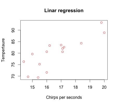
> plot(x,y, main="Linar regression", xlab="Chirps per seconds", ylab="Tempertaure",col="red") # Scatter plot of y against x
>sreg=lm(y~x)                       # Performing simple linear regression of y against x and saving it as " sreg"
> summary(sreg)                     # Obtaining important summary about the regression
Call:
lm(formula = y ~ x)
Residuals:
Min 1Q Median 3Q Max
-6.5041 -1.9044 0.4589 2.7562 5.0222
Coefficients:
Estimate Std. Error t value Pr(>|t|)
(Intercept) 24.8401 10.0227 2.478 0.0277 *
x 3.3158 0.5989 5.536 9.61e-05 ***
---
Signif. codes: 0 ‘***’ 0.001 ‘**’ 0.01 ‘*’ 0.05 ‘.’ 0.1 ‘ ’ 1
Residual standard error: 3.814 on 13 degrees of freedom
Multiple R-squared: 0.7022, Adjusted R-squared: 0.6793
F-statistic: 30.65 on 1 and 13 DF, p-value: 9.606e-05
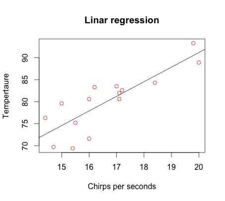
>lines(abline(sreg)) # Fitting the regression line
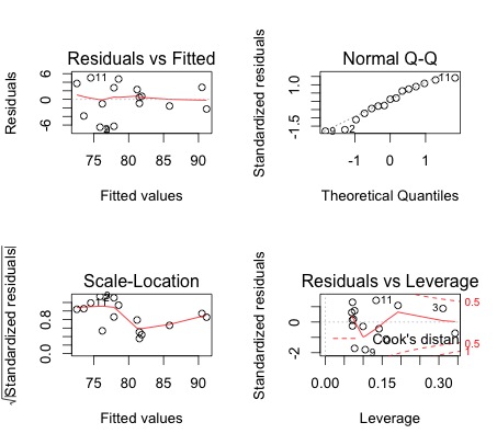
>op=par(mfrow=c(2,2))              # Dividing the plot window into four frames
>plot(sreg)                        # Regression plots and diagnostics
>par(op)                           # Reset to previous .
Interpretation of the results:
- The scatter shows a linea trend: as the frequency increases, so does the temperature. This suggests the existence of a linear relationship between these two variables.
- The summary of the regression suggests that the best line to fit the scatter plot has an equation of the form y=24.8401+3.3158x, that is, a=24.8401, b=3.3158.
- The small p-values (0.0277 and 9.61e-05) suggest the two estimates are significant.
- The coefficient of determination 0.6793, suggests that about 68% of change observed in Temperature is due to change in Frequency.
- A look a the residuals plot suggest minor departure from normality, but also that observations 2 and 11 could be problematic to our model. The question is whether they can be dropped from our model (because of error in data collection) or if they can left in and therefore a robust regression should be performed. To answer, this rule of thumb is to check if their Cooks' distance is larger than 1/n, where n is the number of observations in the data set.
>cd<-cooks.distance(sreg)        # Saving the Cooks' distances in
>Cric1<-cbind(Cric,cd)           # Adding a the column "cd" to the original dataset and crea
>Cric1[cd>4/15,]                 # Displaying the data point whose Cooks distance are deemed large, that is, greater than 1/15