Multiple Linear Regression with R

Data description:

From the article Absorption of Phosphate, Arsenate, Methanearsonate,and Cacodylate by Lake and Sediments: Comparison with Soils (J. of Environ. Quality., 1984:499-504), it is given that Soil and Sediment Absorption, the extent to which chemicals collect in a condensed form of the surface, is an important characteristic because it influeneces the effectivness of the pesticides and various agricultural chemicals.
The file "ssa.txt" describes the phosphate absorption index (PhosphateExtraIndex), the amount of extractable iron(AmountExtraIon) and the amount of extractable aluminum (AmountExtraAlum). It is believed that the phosphate absorption index is linearly dependent on both amounts of extractable iron and aluminum. The data consists of n=13 observations.

Analysis:

>ssa=read.table("file=http://ramanujan.math.trinity.edu/ekwess/misc/ssabsorption.txt", header=TRUE)           # importing the data
into the R workspace and saving it as "ssa"

>head(ssa)                                                                                               # displaying the first rows 

 
AmountExtraIon AmountExtraAlum PhosphateExtraIndex
1             61              13                   4
2            175              21                  18
3            111              24                  14
4            124              23                  18
5            130              64                  26
6            173              38                  26

>x1=ssa$AmountExtraIon                                        # Renaming the variables
>x2=ssa$AmountExtraAlum
>y=ssa$PhosphateExtraIndex
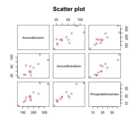
>plot(ssa, main="Scatter Plot",col="red")                     # Multivariate Scatter plot of y against x1 and x2

Click to view


>mreg=lm(y~x1+x2)          # Performing multiple  linear regression of y against the x1 and x2 and saving it as "mreg"
>summary(mreg)             # Obtaining the summary of the multiple linera regression

Call:

lm(formula = y ~ x1 + x2)

Residuals:

    Min      1Q  Median      3Q     Max 

-8.9352 -2.2182  0.4613  3.3448  6.0708 

Coefficients:
            Estimate Std. Error t value Pr(>|t|)    
(Intercept) -7.35066    3.48467  -2.109 0.061101 .  
x1           0.11273    0.02969   3.797 0.003504 ** 
x2           0.34900    0.07131   4.894 0.000628 ***
---
Signif. codes:  0 ‘***’ 0.001 ‘**’ 0.01 ‘*’ 0.05 ‘.’ 0.1 ‘ ’ 1

Residual standard error: 4.379 on 10 degrees of freedom
Multiple R-squared:  0.9485, Adjusted R-squared:  0.9382 
F-statistic: 92.03 on 2 and 10 DF,  p-value: 3.634e-07

>par(mfrow=c(2,2))                   # dividing the plot window into four frames
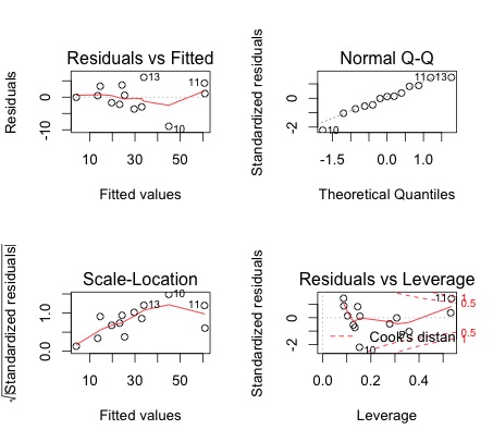
>plot(mreg)                              # Residual plots and diagnostics
>par(op)                             #  End dividing.


Click to view


Interpretation of the results:

  1. The scatter plot shows a linear relationship between the Phosphate Absorption Index, the Amount of Extractable Iron, and the Amount of Extractable Aluminum.
  2. The summary of the regression suggests a relationship of the form y=-7.35066+0.11273x1+0.34900x2.
  3. The small p-values (0.003504 and 0.000628) suggest that the coefficient estimates are highly significant.
  4. The coefficient of determination (0.9382) suggests that about 94% of change in the Phosphate Absorption Index  is due to changes in the Amounts of Extractable Iron and Aluminum respectively.
  5. The normal QQ plots shows that the assumption of normality is valid. The residuals-vs-fitted values-plot does not show a particular pattern, and the vertical spread does not vary too along the horizontal lenght. Moreover, this plot also suggests that the residuals may be centered around 0. Thus it is likely that the assumptions of independence, equal mean 0,  and that of  equal variances (homoscedasticity) are  satisfied.
  6. There are ways to check some of these assumptions individually in R.

Checking Assumptions:

-Normality Test.
There are many normality tests in the package "nortest" that can be performed on the residuals.

>install.packages("nortest")            # Instaling the package "nortest"\
>require(nortest)                       # Loading the package nortest into the R workspace
>res<-mreg$resid                        # saving the residuals from the regression as "res"
>ad.test(res)                           # Anderson-Darling test of normality
>cvm(res)                               # Cramer-Von-Mises test of normality
>lillie.test(res)                       # Kolomogorov-Smirnov test of normality
>sf.test(res)                           # Shapiro-Francia test of normality
>shapiro.test(res)                      # Shapiro test of normalty
>pearson.test(res)                      # Pearson test of normality.
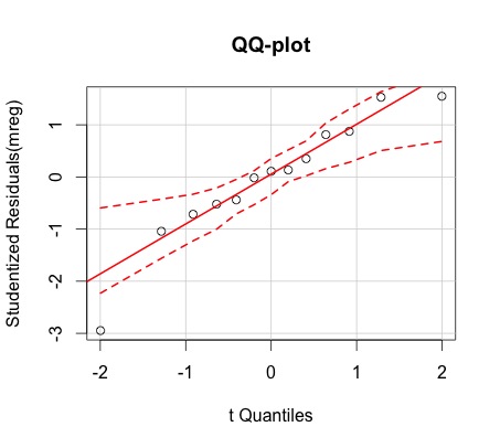

-QQ-plot

>qqp(mreg, envelope=0.95, main="QQ-plot")     # QQplot with an envelope showing a 95%  point-wise confidence level.

Click to view

-Constant Errors Variance test:

>require(car)                         # Loading  the package "car"
> ncvTest(mreg)                       # R tests if the errors have non constant variance.          
 

Non-constant Variance Score Test 
Variance formula: ~ fitted.values 
Chisquare = 1.821239    Df = 1     p = 0.1771659 
Note that the large p-value (0.1771659) indicates that the null hypothesis that the variance are equal is not rejected.

-Independence of errors Test

>durbinWatsonTest(mreg)              # R tests for autocorrelation between the errors. The required packages is "car" 

lag       Autocorrelation    D-W Statistic p-value
  1       -0.4130457          2.633909       0.308
 Alternative hypothesis: rho != 0
Note that the large p-value ( 0.308) indicates the null hypothesis that the correlation coefficient rho  between the errors is equal to zero is not rejected.

Going Further:
You can check the package "nortest" for details on normality tests and these books by John Fox Applied regression analysis and generalized linear models (2nd ed) or  An R and S-Plus companion to applied regression.