Logistic Regression with R

Data description

The data set "ColdWar.txt" located at "http://ramanujan.math.trinity.edu/ekwessi/misc/ColdWar.txt represents the number of ICBMs between the US and USSR years after 1959. 
The question of interest here is to find the relationship (if it exists) between the number of ICBMs (in thousand)  between the US and USSR after  1959 and the year.
 
Analysis


>Cw<-raed.table(file="http://ramanujan.math.trinity.edu/ekwessi/misc/ColdWar.txt", header=T)  #uploading the data into the
 R-workspace.

>head(CW)                         # viewing the first lines of the dataset

 
    Years NumberOfICBM
1     1           18
2     2           63
3     3          294
4     4          424
5     5          854
6     6          854
 

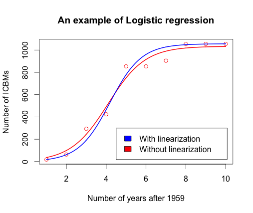
>plot(CW,main="An example of Logistic regression", xlab="Number of years after 1959", ylab="Number of ICBMs",col="red")  # Plot
                   the data to guess the adequate model


>y=CW$NumberOfICBM>x=CW$Years           # appropriately renaming the variables.
>lreg=lm(log((1056-y)/y)~x, data=CW)    # Finding the values of a and b using linearization. L is assumed to be 1056
based on the horizontal asymptote on the scatter plot

>summary(lreg)                          # Summary of the logistic regression

 
Call:
lm(formula = log((1056 - y)/y) ~ x, data = CW)
 
Residuals:
     Min       1Q   Median       3Q      Max 
-1.41888 -0.52019 -0.01118  0.36296  1.79373 
 
Coefficients:
            Estimate Std. Error t value Pr(>|t|)    
(Intercept)   5.3248     0.6558   8.119 3.92e-05 ***
x            -1.2716     0.1057 -12.031 2.10e-06 ***
---
Signif. codes:  0 ‘***’ 0.001 ‘**’ 0.01 ‘*’ 0.05 ‘.’ 0.1 ‘ ’ 1
 
Residual standard error: 0.96 on 8 degrees of freedom
Multiple R-squared:  0.9476, Adjusted R-squared:  0.9411 
F-statistic: 144.8 on 1 and 8 DF,  p-value: 2.102e-06
 

>t=seq(1,length(x),0.01)
>z=1056/(1+exp(lreg$coef[1]+lreg$coef[2]*t))
>lines(t,z,type="l",col="blue", lwd=2)                  #Fitting the model into the data

 
Remark
1. The plot seems to indicate that the logistic model is suitable to predict the number of ICBMs between the US and USSR years after the year 1959.
2. The Adjusted-R-squared (0.9411) indicates that over the next 10 years after 159, changes in the number of ICBMs can well be explained using the logistic model.
2. The values of a and b can also  be found using the Gauss-Newton algorithm. We can then compare the two models and use the AIC or BIC for model selection.


>lreg2=nls(y~L/(1+exp(a+b*x)),start=list(a=5,b=-1,L=1044),data=CW)  # Using nonlinear regression to find the regression
coefficients a, b and L.

>summary(lreg2)

 
Formula: y ~ L/(1 + exp(a + b * x))
 
Parameters:
   Estimate Std. Error t value Pr(>|t|)    
a    4.3900     0.7336   5.984 0.000551 ***
b   -1.0730     0.1869  -5.741 0.000705 ***
L 1033.3655    39.5050  26.158 3.05e-08 ***
---
Signif. codes:  0 ‘***’ 0.001 ‘**’ 0.01 ‘*’ 0.05 ‘.’ 0.1 ‘ ’ 1
 
Residual standard error: 68.7 on 7 degrees of freedom
 
Number of iterations to convergence: 8 
Achieved convergence tolerance: 2.812e-06


> AIC(lreg,lreg2)      # Comparing the two models using their AIC.

 
 df       AIC
lreg   3  31.33129
lreg2  4 117.40583


>u=seq(1,length(x),0.01)
>v=1033.3655/(1+exp(4.39-1.0730*u))
>lines(u,v,type="l",col="red", lwd=2)
>legend(6,200,c("Assuming L=1056","Without assumptions on L"), fill=c("blue","red"))   # Overlaying the two models on the same
graph